The lowest point in the western hemisphere is found in California's Death Valley National Park, at a location called
Badwater Basin. At that location, one can stand on ground which is 86 meters (282 feet) below sea level!
If the Statue of Liberty were placed atop her pedestal at this location, and then Death Valley were filled with
water up to sea level, and only the very top of Lady Liberty's torch would poke up above the water!
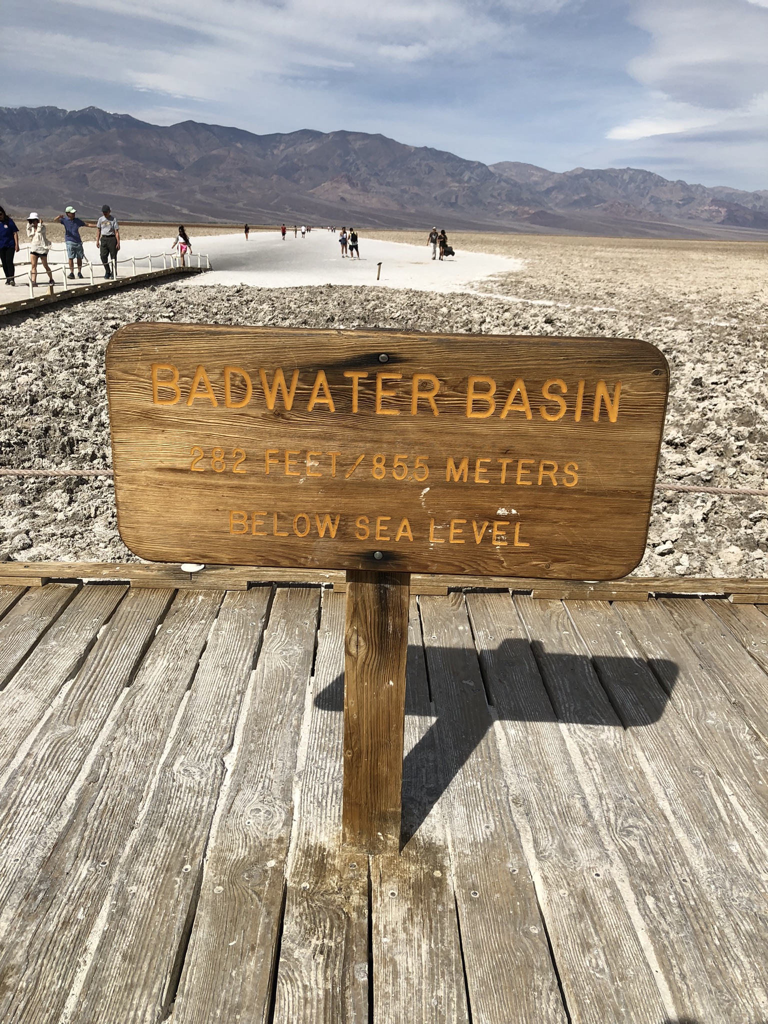
Photo by Daniel Stober, © 2022
All of that below sea level stuff is interesting to me as a geography nerd, but the purpose of this page is to demonsytrate how to integrate SVG elements into your Leaflet maps. In particular, I want focus on the code needed to place an svg object onto the map and the challenges inherent in positioning the SVG at the proper location on the map.
When it comes to positioning, the biggest challenge to overcome is that the two technologies utilize different base units: Leaflet, and mapping in general, are based in latitude and logitude, while SVG is built in pixels. This presents difficulties in precise positioning, especially when users can alter the zoom level of the map -- which then changes the number of pixels between points in the display.
Map 1: Getting Started - Leaflet marker and positioning
To start, I'll show you a map that uses the standard Leaflet marker library. The marker is positioned so that the bottom point of the marker is the location pinpointed. In this case, the pinpoint is at 36.230°N 116.768°W, which is the location of Badwater Basin, the lowest point in the western hemisphere.
Map 1
This map is generated with javascript function map1( ){ }Use the controls to zoom in and out on the map; Notice that the image icon positioning on the map is adjusted to ensure that the pinpointed location remains the same, even if you move the map around so that the pinpointed location is not centered.
let map_attribution = 'Map data © <a href="https://www.openstreetmap.org/">OpenStreetMap</a> contributors, ' +
'<a href="https://creativecommons.org/licenses/by-sa/2.0/">CC-BY-SA</a>, ' +
'Imagery © >a href="https://www.openstreetmap.org/copyright" target="_0"<OpenStreetMap>/a<'
let badwater_coords = [36.230, -116.768]
let map = L.map('map1').setView( badwater_coords, 10);
L.tileLayer( URL, { attribution: map_attribution } ).addTo(map);
// Place a marker at Badwater
L.marker( badwater_coords ).addTo(map);
The code above is the minimal javascript code required to generate Map 1.
The first two statements declare that the map will be using the tile set from Open Street Map (OSM),so the URL and other additional information is written to a couple of variables.
Below that, I have hardcoded the desired latitude and longitude into a variable which is an array object (square brackets) and then declared an instance of a Leaflet map centered on that point. The same variablewill be reused to place a Leaflet marker on that spot.
Next, comes the call which adds the tileset to the map. The tileset is the set of images files that make a map look like, well, a map! As I mentioned above, the URL for this tileset was writtent to a variable.
All of the above code will be used on all of the subsequent maps on this page, too.
Finally, the code places a Leaflet marker at the location
The text included for map attribution may look like superfluous code, but the terms and conditions for use of
both the free Leaflet libraries and open source maps require that you include attribution when you use them, so
please don't overlook it.
One more thing to note is that the Leaflet javascript libraries must be imported onto your page in order to be used in the javascript
demonstrated here. That takes place at the very top of the HTML, in the <head> section of the page, where you will find this:
<link rel="stylesheet" href="https://unpkg.com/leaflet@1.7.1/dist/leaflet.css"/>
<script src="https://unpkg.com/leaflet@1.7.1/dist/leaflet.js"></script>
Strictly speaking, the link to the Google fonts is not necessary, but it allows me to use those fonts.
Map 2: Adding an SVG element to the map
In the next map, I have added an SVG palette and placed two shapes onto it. To make easier to digest the spatial
relationship, I left the Leaflet marker from the previous map on the page. The Leaflet marker is still pointing to
the true location of Badwater, but the SVG markers leave something to be desired.
So, first of all, let's take a look at the SVG object:
This is a complete SVG document which creates one circle and two squares. (See the SVG document
here.) The squares are actually <rect> objects
with widths equal to their heights. The black rect is 100 pixels by 100 pixels, which is the size of the SVG canvass itself. The
red rect is only 40 by 40, while the circle has a radius of 20 pixels.
The first thing that may jump out is that you can see only one quarter of the circle. The other three-quarters have spilled off
the canvass. This is because the center of the circle, defined by the values attributes "cx" and "cy", is at position (0,0), which is
at the upper left hand corner of the canvass. It's easy to imagine a complete circle there with the other quadrants running off of the
canvass.
On the other hand, <rect> objects are defined based on the location of their "x" and "y" attributes. In these cases, again, that
is position (0,0), but for these objects position (0,0) is the location of the upper left hand corner of the shape, so these
<rect> objects appear fully on the canvass; the red one is 40 pixels across and 40 pixels down while is black one is 100 pixels
across and down.
The black one, however, provides two important clues to how we can position these objects. We know that the SVG object is 100 pixels wide
by 100 pixels tall. How do we know that? Because it defined as such in this Leaflet statement:
When a <rect> object with identical dimensions is placed onto the palette, we get insight into how the SVG object is positioned onto the map. The center of the black square is precisely positioned at the GPS coordinates of Badwater, we can tell that because the Leaflet marker is still on the map. Further, we know that the SVG icon was positioned at the location of Badwater, in this statement.
It is that statement which adds the SVG to the map. The location is specified in the first parameter which references the same variable used
to position the Leaflet marker, "badwater_coords." The "icon" is the SVG document itself. From this, we can infer that the location
specifed when the SVG document is placed onto the map is the center point of the SVG canvass. In this case, the location of Badwater concides
with position (50,50) on the SVG. We now have a way to align the pixels of the SVG with the latitude and longitude grid of the map.
To see the big picture, combine the statements from Map 1 with the following statements to see the complete document used to build this map.
svgDocument = "<svg xmlns='http://www.w3.org/2000/svg'>"
+ "<circle cx='0' cy='0' r='20' fill='rgba(255,215,0,0.5)' stroke='green' stroke-width='1px'></circle>"
+ "<rect x='0' y='0' width='40' height='40' stroke='red' stroke-width='1px' fill='none'></rect>"
+ "<rect x='0' y='0' width='100' height='100' stroke='black' stroke-width='1px' fill='none'></rect>"
+"</svg>";
svgUri = encodeURI("data:image/svg+xml," + svgDocument );
svgIcon = new CustomIcon ( {iconUrl: svgUri });
// The center of the SVG icon is at the lat/long specified at L.marker
L.marker( badwater_coords, {icon: svgIcon} ).addTo ( map );
You can also all of these statements together by looking at function map2() in the source code.
If you want to see the SVG document by itself (without the map), click here.
Map 2
function map2( ){ }Map 3: Positioning SVG elements on a point
You may have hoped that there would be no math in this demostration, but we'll need just a little bit of grade school cyphering to
for precise placement of SVG objects on the map.
What we know:
- The SVG canvass is 100 by 100
- The centerpoint of the SVG is located at the plotted GPS location.
- The centerpoint of the canvass is at plot point (50,50)
- To be centered, objects on the canvass must extend equal distances above and below the midpoint and equal distances left and right of the midpoint
To center a circle on the SVG canvass, the circle's centerpoint must coincide with the centerpoint of the canvass. No math needed for this one: The circle's centerpoint, specified by attributes "cx" and "cy", will be (50,50).
<circle cx='50' cy='50' r='20' fill='rgba(255,215,0,0.5)' stroke='green' stroke-width='1px'></circle>
<rect x='30' y='30' width='40' height='40' stroke='red' stroke-width='1px' fill='none'></rect>
<rect x='0' y='0' width='100' height='100' stroke='black' stroke-width='1px' fill='none'></rect>
</svg>
Now take a look at Map 3, we can see that we have now centered a circle and a square on the Badwater point
While I was tempted to refactor the javascript code and reuse common elements among the maps, I resisted that temptation so that you can
go to the source and have complete code that will run simply by cutting and pasting. Please feel free to grabd it and modify it as you
see fit.
In one final map, I have placed a JPEG image on the map in the same manner as a SVG. Even though the JPEG referenced is 750 by 1000 pixels, it
get collapsed down to 90 x 120 by this statement.
iconUrl: 'images\\badwater_IMG_8716.JPEG',
iconSize: [90, 120]
}
Luckily I don't have to do any math to center the photo over the location of Badwater. In much the same way that an SVG is automatically centered, so too is an image centered.
Stay tuned for a future post which will take this concept to the next left -- I'll show you how to add mulitple SVG objects and coordinate them with a single <g> element. It's trickier than you might think.
Maps and text on this page ©2023 by Daniel Stober. All rights reserved.
Cartography from Open Street Map
Last Updated 2023-03-04
Back to Carto Dan page
Back to DanStober.net